Microsoft Excel provides a special MONTH function to extract a month from date, which returns the month number ranging from 1 (January) to 12 (December).
The MONTH function can be used in all versions of Excel 2013 - 2000 and its syntax is as simple as it can possibly be:
MONTH(serial_number)
Where serial_number is any valid date of the month you are trying to find.
For the correct work of Excel MONTH formulas, a date should be entered by using the DATE(year, month, day) function. For example, the formula =MONTH(DATE(2015,3,1)) returns 3 since DATE represents the 1st day of March, 2015.
Formulas like =MONTH("1-Mar-2015") also work fine, though problems may occur in more complex scenarios if dates are entered as text.
In practice, instead of specifying a date within the MONTH function, it's more convenient to refer to a cell with a date or supply a date returned by some other function. For example:
=MONTH(A1) - returns the month of a date in cell A1.
=MONTH(TODAY()) - returns the number of the current month.
At first sight, the Excel MONTH function may look plain. But look through the below examples and you will be amazed to know how many useful things it can actually do.
How to get month number from date in Excel
There are several ways to get month from date in Excel. Which one to choose depends on exactly what result you are trying to achieve.
1. MONTH function in Excel - get month number from date.
This is the most obvious and easiest way to convert date to month in Excel. For example:
=MONTH(A2) - returns the month of a date in cell A2.
=MONTH(DATE(2015,4,15)) - returns 4 corresponding to April.
=MONTH("15-Apr-2015") - obviously, returns number 4 too.
2. TEXT function in Excel - extract month as a text string.
An alternative way to get a month number from an Excel date is using the TEXT function:
=TEXT(A2, "m") - returns a month number without a leading zero, as 1 - 12.
=TEXT(A2,"mm") - returns a month number with a leading zero, as 01 - 12.
Please be very careful when using TEXT formulas, because they always return month numbers as text strings. So, if you plan to perform some further calculations or use the returned numbers in other formulas, you'd better stick with the Excel MONTH function.
The following screenshot demonstrates the results returned by all of the above formulas. Please notice the right alignment of numbers returned by the MONTH function (cells C2 and C3) as opposed to left-aligned text values returned by the TEXT functions (cells C4 and C5).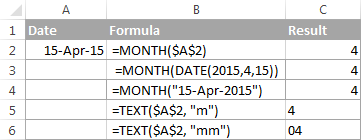
How to extract month name from date in Excel
In case you want to get a month name rather than a number, you use the TEXT function again, but with a different date code:
=TEXT(A2, "mmm") - returns an abbreviated month name, as Jan - Dec.
=TEXT(A2,"mmmm") - returns a full month name, as January - December.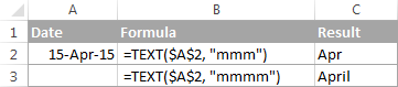
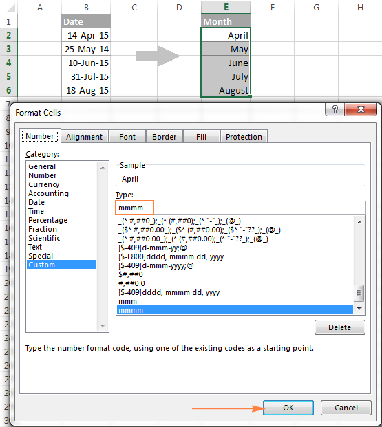
If you don't actually want to convert date to month in your Excel worksheet, you are just wish todisplay a month name only instead of the full date, then you don't want any formulas.
Select a cell(s) with dates, press Ctrl+1 to opent the Format Cells dialog. On the Number tab, selectCustom and type either "mmm" or "mmmm" in the Type box to display abbreviated or full month names, respectively. In this case, your entries will remain fully functional Excel dates that you can use in calculations and other formulas. For more details about changing the date format, please see Creating a custom date format in Excel.
How to convert month number to month name in Excel
Suppose, you have a list of numbers (1 through 12) in your Excel worksheet that you want to convert to month names. To do this, you can use any of the following formulas:
1. To return an abbreviated month name (Jan - Dec).
=TEXT(A2*28, "mmm")
=TEXT(DATE(2015, A2, 1), "mmm")
2. To return a full month name (January - December).
=TEXT(A2*28, "mmmm")
=TEXT(DATE(2015, A2, 1), "mmmm")
In all of the above formulas, A2 is a cell with a month number. And the only real difference between the formulas is the month codes:
"mmm" - 3-letter abbreviation of the month, such as Jan - Dec
"mmmm" - month spelled out completely
"mmmmm" - the first letter of the month name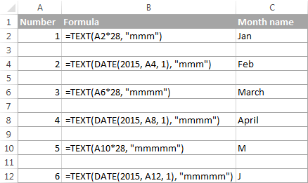
How to convert month name to number in Excel
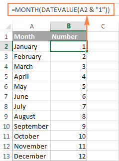
There are two Excel functions that can help you convert month names to numbers - DATEVALUE and MONTH. Excel's DATEVALUE function converts a date stored as text to a serial number that Microsoft Excel recognizes as a date. And then, the MONTH function extracts a month number from that date.
The complete formula is as follows:
=MONTH(DATEVALUE(A2 & "1"))
Where A2 in a cell containing the month name you want to turn into a number (&"1" is added for the DATEVALUE function to understand it's a date).
Example 2. Get the 1st day of month from a date
If you want to calculate the first day of the month based on a date, you can use the Excel DATE function again, but this time you will also need the MONTH function to extract the month number:
=DATE(year, MONTH(cell with the date), 1)
For example, the following formula will return the first day of the month based on the date in cell A2:
=DATE(2015,MONTH(A2),1)
Example 3. Find the first day of month based on the current date
When your calculations are based on today's date, use a liaison of the Excel EOMONTH and TODAY functions:
=EOMONTH(TODAY(),0) +1 - returns the 1st day of the following month.
As you remember, we already used a similar EOMONTH formula to get the last day of the current month. And now, you simply add 1 to that formula to get the first day of the next month.
In a similar manner, you can get the first day of the previous and current month:
=EOMONTH(TODAY(),-2) +1 - returns the 1st day of the previous month.
=EOMONTH(TODAY(),-1) +1 - returns the 1st day of the current month.
You could also use the Excel DATE function to handle this task, though the formulas would be a bit longer. For example, guess what the following formula does?
=DATE(YEAR(TODAY()), MONTH(TODAY()), 1)
Yep, it returns the first day of the current month.
And how do you force it to return the first day of the following or previous month? Hands down :) Just add or subtract 1 to/from the current month:
To return the first day of the following month:
=DATE(YEAR(TODAY()), MONTH(TODAY())+1, 1)
To return the first day of the previous month:
=DATE(YEAR(TODAY()), MONTH(TODAY())-1, 1)
How to calculate the number of days in a month
In Microsoft Excel, there exist a variety of functions to work with dates and times. However, it lacks a function for calculating the number of days in a given month. So, we'll need to make up for that omission with our own formulas.
Example 1. To get the number of days based on the month number
If you know the month number, the following DAY / DATE formula will return the number of days in that month:
=DAY(DATE(year, month number + 1, 1) -1)
In the above formula, the DATE function returns the first day of the following month, from which you subtract 1 to get the last day of the month you want. And then, the DAY function converts the date to a day number.
For example, the following formula returns the number of days in April (the 4th month in the year).
=DAY(DATE(2015, 4 +1, 1) -1)
Example 2. To get the number of days in a month based on date
If you don't know a month number but have any date within that month, you can use the YEAR and MONTH functions to extract the year and month number from the date. Just embed them in the DAY / DATE formula discussed in the above example, and it will tell you how many days a given month contains:
=DAY(DATE(YEAR(A2), MONTH(A2) +1, 1) -1)
Where A2 is cell with a date.
Alternatively, you can use a much simpler DAY / EOMONTH formula. As you remember, the Excel EOMONTH function returns the last day of the month, so you don't need any additional calculations:
=DAY(EOMONTH(A1, 0))
The following screenshot demonstrates the results returned by all of the formulas, and as you see they are identical:
How to sum data by month in Excel
In a large table with lots of data, you may often need to get a sum of values for a given month. And this might be a problem if the data was not entered in chronological order.
The easiest solution is to add a helper column with a simple Excel MONTH formula that will convert dates to month numbers. Say, if your dates are in column A, you use =MONTH(A2).
And now, write down a list of numbers (from 1 to 12, or only those month numbers that are of interest to you) in an empty column, and sum values for each month using a SUMIF formula similar to this:
=SUMIF(C2:C15, E2, B2:B15)
Where E2 is the month number.
The following screenshot shows the result of the calculations: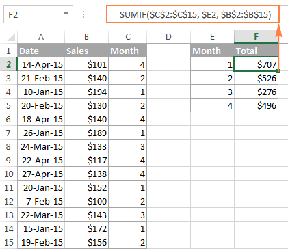
If you'd rather not add a helper column to your Excel sheet, no problem, you can do without it. A bit more trickier SUMPRODUCT function will work a treat:
=SUMPRODUCT((MONTH($A$2:$A$15)=$E2) * ($B$2:$B$15))
Where column A contains dates, column B contains the values to sum and E2 is the month number.
Note. Please keep in mind that both of the above solutions add up all values for a given month regardless of the year. So, if your Excel worksheet contains data for several years, all of it will be summed.
How to conditionally format dates based on month
Now that you know how to use the Excel MONTH and EOMONTH functions to perform various calculations in your worksheets, you may take a step further and improve the visual presentation. For this, we are going to use the capabilities of Excel conditional formatting for dates.
In addition to the examples provided in the above mentioned article, now I will show you how you can quickly highlight all cells or entire rows related to a certain month.
Example 1. Highlight dates within the current month
In the table from the previous example, suppose you want to highlight all rows with the current month dates.
First off, you extract the month numbers from dates in column A using the simplest =MONTH($A2) formula. And then, you compare those numbers with the current month returned by =MONTH(TODAY()). As a result, you have the following formula which returns TRUE if the months' numbers match, FALSE otherwise:
=MONTH($A2)=MONTH(TODAY())
Create an Excel conditional formatting rule based on this formula, and your result may resemble the screenshot below (the article was written in April, so all April dates are highlighted).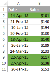
Example 2. Highlighting dates by month and day
And here's another challenge. Suppose you want to highlight the major holidays in your worksheet regardless of the year. Let's say Christmas and New Year days. How would you approach this task?
Simply use the Excel DAY function to extract the day of the month (1 - 31) and the MONTH function to get the month number, and then check if the DAY is equal to either 25 or 31, and if the MONTH is equal to 12:
=AND(OR(DAY($A2)=25, DAY($A2)=31), MONTH(A2)=12)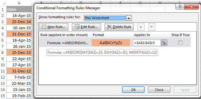
Source : https://www.ablebits.com/office-addins-blog/2015/04/22/excel-month-eomonth-functions/
The MONTH function can be used in all versions of Excel 2013 - 2000 and its syntax is as simple as it can possibly be:
MONTH(serial_number)
Where serial_number is any valid date of the month you are trying to find.
For the correct work of Excel MONTH formulas, a date should be entered by using the DATE(year, month, day) function. For example, the formula =MONTH(DATE(2015,3,1)) returns 3 since DATE represents the 1st day of March, 2015.
Formulas like =MONTH("1-Mar-2015") also work fine, though problems may occur in more complex scenarios if dates are entered as text.
In practice, instead of specifying a date within the MONTH function, it's more convenient to refer to a cell with a date or supply a date returned by some other function. For example:
=MONTH(A1) - returns the month of a date in cell A1.
=MONTH(TODAY()) - returns the number of the current month.
At first sight, the Excel MONTH function may look plain. But look through the below examples and you will be amazed to know how many useful things it can actually do.
How to get month number from date in Excel
There are several ways to get month from date in Excel. Which one to choose depends on exactly what result you are trying to achieve.
1. MONTH function in Excel - get month number from date.
This is the most obvious and easiest way to convert date to month in Excel. For example:
=MONTH(A2) - returns the month of a date in cell A2.
=MONTH(DATE(2015,4,15)) - returns 4 corresponding to April.
=MONTH("15-Apr-2015") - obviously, returns number 4 too.
2. TEXT function in Excel - extract month as a text string.
An alternative way to get a month number from an Excel date is using the TEXT function:
=TEXT(A2, "m") - returns a month number without a leading zero, as 1 - 12.
=TEXT(A2,"mm") - returns a month number with a leading zero, as 01 - 12.
Please be very careful when using TEXT formulas, because they always return month numbers as text strings. So, if you plan to perform some further calculations or use the returned numbers in other formulas, you'd better stick with the Excel MONTH function.
The following screenshot demonstrates the results returned by all of the above formulas. Please notice the right alignment of numbers returned by the MONTH function (cells C2 and C3) as opposed to left-aligned text values returned by the TEXT functions (cells C4 and C5).
How to extract month name from date in Excel
In case you want to get a month name rather than a number, you use the TEXT function again, but with a different date code:
=TEXT(A2, "mmm") - returns an abbreviated month name, as Jan - Dec.
=TEXT(A2,"mmmm") - returns a full month name, as January - December.
If you don't actually want to convert date to month in your Excel worksheet, you are just wish todisplay a month name only instead of the full date, then you don't want any formulas.
Select a cell(s) with dates, press Ctrl+1 to opent the Format Cells dialog. On the Number tab, selectCustom and type either "mmm" or "mmmm" in the Type box to display abbreviated or full month names, respectively. In this case, your entries will remain fully functional Excel dates that you can use in calculations and other formulas. For more details about changing the date format, please see Creating a custom date format in Excel.
How to convert month number to month name in Excel
Suppose, you have a list of numbers (1 through 12) in your Excel worksheet that you want to convert to month names. To do this, you can use any of the following formulas:
1. To return an abbreviated month name (Jan - Dec).
=TEXT(A2*28, "mmm")
=TEXT(DATE(2015, A2, 1), "mmm")
2. To return a full month name (January - December).
=TEXT(A2*28, "mmmm")
=TEXT(DATE(2015, A2, 1), "mmmm")
In all of the above formulas, A2 is a cell with a month number. And the only real difference between the formulas is the month codes:
"mmm" - 3-letter abbreviation of the month, such as Jan - Dec
"mmmm" - month spelled out completely
"mmmmm" - the first letter of the month name
How to convert month name to number in Excel
There are two Excel functions that can help you convert month names to numbers - DATEVALUE and MONTH. Excel's DATEVALUE function converts a date stored as text to a serial number that Microsoft Excel recognizes as a date. And then, the MONTH function extracts a month number from that date.
The complete formula is as follows:
=MONTH(DATEVALUE(A2 & "1"))
Where A2 in a cell containing the month name you want to turn into a number (&"1" is added for the DATEVALUE function to understand it's a date).
How to get the last day of month in Excel (EOMONTH function)
The EOMONTH function in Excel is used to return the last day of the month based on the specified start date. It has the following arguments, both of which are required:
EOMONTH(start_date, months)
Start_date - the starting date or a reference to a cell with the start date.
Months - the number of months before or after the start date. Use a positive value for future dates and negative value for past dates.
Here are a few EOMONTH formula examples:
=EOMONTH(A2, 1) - returns the last day of the month, one month after the date in cell A2.
=EOMONTH(A2, -1) - returns the last day of the month, one month before the date in cell A2.
Instead of a cell reference, you can hardcode a date in your EOMONTH formula. For example, both of the below formulas return the last day in April.
=EOMONTH("15-Apr-2015", 0)
=EOMONTH(DATE(2015,4,15), 0)
To return the last day of the current month, you use the TODAY() function in the first argument of your EOMONTH formula so that today's date is taken as the start date. And, you put 0 in the months argument because you don't want to change the month either way.
=EOMONTH(TODAY(), 0)
Note. Since the Excel EOMONTH function returns the serial number representing the date, you have to apply the date format to a cell(s) with your formulas. Please see How to change date format in Excel for the detailed steps.
And here are the results returned by the Excel EOMONTH formulas discussed above: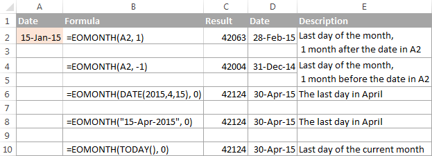
If you want to calculate how many days are left till the end of the current month, you simply subtract the date returned by TODAY() from the date returned by EOMONTH and apply the General format to a cell:
=EOMONTH(TODAY(), 0)-TODAY()
How to find the first day of month in Excel
As you already know, Microsoft Excel provides just one function to return the last day of the month (EOMONTH). When it comes to the first day of the month, there is more than one way to get it.
Example 1. Get the 1st day of month by the month number
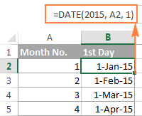
If you have the month number, then use a simple DATE formula like this:
=DATE(year, month number, 1)
For example, =DATE(2015, 4, 1) will return 1-Apr-15.
If your numbers are located in a certain column, say in column A, you can add a cell reference directly in the formula:
=DATE(2015, B2, 1)
The EOMONTH function in Excel is used to return the last day of the month based on the specified start date. It has the following arguments, both of which are required:
EOMONTH(start_date, months)
Start_date - the starting date or a reference to a cell with the start date.
Months - the number of months before or after the start date. Use a positive value for future dates and negative value for past dates.
Here are a few EOMONTH formula examples:
=EOMONTH(A2, 1) - returns the last day of the month, one month after the date in cell A2.
=EOMONTH(A2, -1) - returns the last day of the month, one month before the date in cell A2.
Instead of a cell reference, you can hardcode a date in your EOMONTH formula. For example, both of the below formulas return the last day in April.
=EOMONTH("15-Apr-2015", 0)
=EOMONTH(DATE(2015,4,15), 0)
To return the last day of the current month, you use the TODAY() function in the first argument of your EOMONTH formula so that today's date is taken as the start date. And, you put 0 in the months argument because you don't want to change the month either way.
=EOMONTH(TODAY(), 0)
Note. Since the Excel EOMONTH function returns the serial number representing the date, you have to apply the date format to a cell(s) with your formulas. Please see How to change date format in Excel for the detailed steps.
And here are the results returned by the Excel EOMONTH formulas discussed above:
If you want to calculate how many days are left till the end of the current month, you simply subtract the date returned by TODAY() from the date returned by EOMONTH and apply the General format to a cell:
=EOMONTH(TODAY(), 0)-TODAY()
How to find the first day of month in Excel
As you already know, Microsoft Excel provides just one function to return the last day of the month (EOMONTH). When it comes to the first day of the month, there is more than one way to get it.
Example 1. Get the 1st day of month by the month number
If you have the month number, then use a simple DATE formula like this:
=DATE(year, month number, 1)
For example, =DATE(2015, 4, 1) will return 1-Apr-15.
If your numbers are located in a certain column, say in column A, you can add a cell reference directly in the formula:
=DATE(2015, B2, 1)
Example 2. Get the 1st day of month from a date
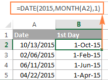
If you want to calculate the first day of the month based on a date, you can use the Excel DATE function again, but this time you will also need the MONTH function to extract the month number:
=DATE(year, MONTH(cell with the date), 1)
For example, the following formula will return the first day of the month based on the date in cell A2:
=DATE(2015,MONTH(A2),1)
Example 3. Find the first day of month based on the current date
When your calculations are based on today's date, use a liaison of the Excel EOMONTH and TODAY functions:
=EOMONTH(TODAY(),0) +1 - returns the 1st day of the following month.
As you remember, we already used a similar EOMONTH formula to get the last day of the current month. And now, you simply add 1 to that formula to get the first day of the next month.
In a similar manner, you can get the first day of the previous and current month:
=EOMONTH(TODAY(),-2) +1 - returns the 1st day of the previous month.
=EOMONTH(TODAY(),-1) +1 - returns the 1st day of the current month.
You could also use the Excel DATE function to handle this task, though the formulas would be a bit longer. For example, guess what the following formula does?
=DATE(YEAR(TODAY()), MONTH(TODAY()), 1)
Yep, it returns the first day of the current month.
And how do you force it to return the first day of the following or previous month? Hands down :) Just add or subtract 1 to/from the current month:
To return the first day of the following month:
=DATE(YEAR(TODAY()), MONTH(TODAY())+1, 1)
To return the first day of the previous month:
=DATE(YEAR(TODAY()), MONTH(TODAY())-1, 1)
How to calculate the number of days in a month
In Microsoft Excel, there exist a variety of functions to work with dates and times. However, it lacks a function for calculating the number of days in a given month. So, we'll need to make up for that omission with our own formulas.
Example 1. To get the number of days based on the month number
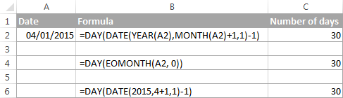
If you know the month number, the following DAY / DATE formula will return the number of days in that month:
=DAY(DATE(year, month number + 1, 1) -1)
In the above formula, the DATE function returns the first day of the following month, from which you subtract 1 to get the last day of the month you want. And then, the DAY function converts the date to a day number.
For example, the following formula returns the number of days in April (the 4th month in the year).
=DAY(DATE(2015, 4 +1, 1) -1)
Example 2. To get the number of days in a month based on date
If you don't know a month number but have any date within that month, you can use the YEAR and MONTH functions to extract the year and month number from the date. Just embed them in the DAY / DATE formula discussed in the above example, and it will tell you how many days a given month contains:
=DAY(DATE(YEAR(A2), MONTH(A2) +1, 1) -1)
Where A2 is cell with a date.
Alternatively, you can use a much simpler DAY / EOMONTH formula. As you remember, the Excel EOMONTH function returns the last day of the month, so you don't need any additional calculations:
=DAY(EOMONTH(A1, 0))
The following screenshot demonstrates the results returned by all of the formulas, and as you see they are identical:
How to sum data by month in Excel
In a large table with lots of data, you may often need to get a sum of values for a given month. And this might be a problem if the data was not entered in chronological order.
The easiest solution is to add a helper column with a simple Excel MONTH formula that will convert dates to month numbers. Say, if your dates are in column A, you use =MONTH(A2).
And now, write down a list of numbers (from 1 to 12, or only those month numbers that are of interest to you) in an empty column, and sum values for each month using a SUMIF formula similar to this:
=SUMIF(C2:C15, E2, B2:B15)
Where E2 is the month number.
The following screenshot shows the result of the calculations:
If you'd rather not add a helper column to your Excel sheet, no problem, you can do without it. A bit more trickier SUMPRODUCT function will work a treat:
=SUMPRODUCT((MONTH($A$2:$A$15)=$E2) * ($B$2:$B$15))
Where column A contains dates, column B contains the values to sum and E2 is the month number.
Note. Please keep in mind that both of the above solutions add up all values for a given month regardless of the year. So, if your Excel worksheet contains data for several years, all of it will be summed.
How to conditionally format dates based on month
Now that you know how to use the Excel MONTH and EOMONTH functions to perform various calculations in your worksheets, you may take a step further and improve the visual presentation. For this, we are going to use the capabilities of Excel conditional formatting for dates.
In addition to the examples provided in the above mentioned article, now I will show you how you can quickly highlight all cells or entire rows related to a certain month.
Example 1. Highlight dates within the current month
In the table from the previous example, suppose you want to highlight all rows with the current month dates.
First off, you extract the month numbers from dates in column A using the simplest =MONTH($A2) formula. And then, you compare those numbers with the current month returned by =MONTH(TODAY()). As a result, you have the following formula which returns TRUE if the months' numbers match, FALSE otherwise:
=MONTH($A2)=MONTH(TODAY())
Create an Excel conditional formatting rule based on this formula, and your result may resemble the screenshot below (the article was written in April, so all April dates are highlighted).
Example 2. Highlighting dates by month and day
And here's another challenge. Suppose you want to highlight the major holidays in your worksheet regardless of the year. Let's say Christmas and New Year days. How would you approach this task?
Simply use the Excel DAY function to extract the day of the month (1 - 31) and the MONTH function to get the month number, and then check if the DAY is equal to either 25 or 31, and if the MONTH is equal to 12:
=AND(OR(DAY($A2)=25, DAY($A2)=31), MONTH(A2)=12)
No comments:
Post a Comment